
A smooth gradient looks simple, but it can be surprisingly difficult to compress. Small errors that disappear inside a detailed texture become visible as bands, color shifts, and block boundaries against a smooth background.
The key is how a format represents change: BC1 selects from a small color palette; ETC2 can instead describe a spatial color ramp. BC5, BC7, and ASTC offer different ways to improve precision or flexibility.
BC1 versus ETC2#
These are actual encoded and decoded images, not simulated artifacts. The source is a gently varying, two-dimensional RGB gradient. Toggle Absolute error ×16 to expose small differences, then magnify the same crop to inspect individual blocks.

RMSE 0.00

RMSE 2.31

RMSE 2.43

RMSE 0.92
Full 192×192 images. RMSE is measured in 8-bit RGB code values; lower is better. Scroll horizontally on narrow screens to compare all columns.
BC1 and ETC2 RGB both encode a 4×4 block into 64 bits: 4 bits per texel. Yet ETC2 is noticeably closer here. Why?
BC1 Limitations#
For an opaque block in four-color mode, BC1 stores:
- Two RGB565 endpoints: 5 bits red, 6 green, 5 blue each.
- Two more colors interpolated approximately one-third and two-thirds between them.
- A 2-bit index per texel, selecting one of those four colors.
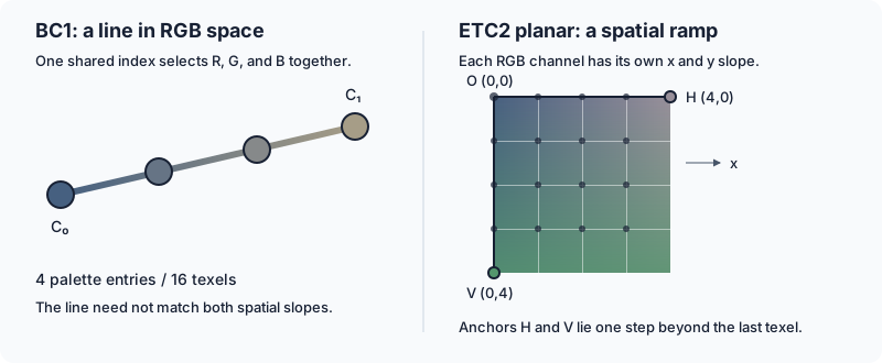
All four colors lie on a single line in RGB space. This creates two distinct limitations:
- Coarse endpoints. A shallow gradient may change by only a few code values across a block, while the endpoint grid has roughly 8-value steps in red/blue and 4 in green. The encoder must compromise, sometimes introducing a color cast.
- A small, shared palette. Sixteen texels share at most four colors. If RGB changes in different directions along the image’s x and y axes, one color line cannot represent the block’s color distribution exactly—even with perfect endpoints.
Neighboring blocks make those compromises independently, exposing their boundaries. Four-color BC1 can still represent some simple ramps well; it does not inevitably fail on every gradient. Its alternative three-color/transparent mode does not provide a larger RGB palette.
ETC2’s Advantage#
For this example, yes: the source image is 192×192 texels. With ETC2’s 4×4 blocks, that gives $(192/4)\times(192/4)=48\times48=2{,}304$ blocks in total. Inspecting the compressed data shows that all 2,304 blocks (100%) use planar mode. RGB RMSE falls from 2.31 for BC1 to 0.92 for ETC2 in 8-bit code values.
The ETC1 comparison is useful: without ETC2’s new modes, error is 2.43 in this test. That isolates the practical benefit here, although these numbers describe these encoders and this image—not a universal ranking.
ETC1 Modes#
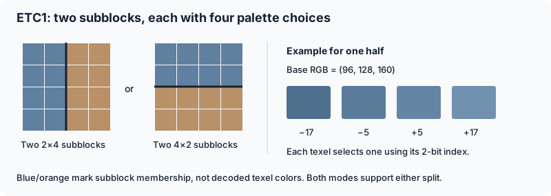
ETC1 also stores a 4×4 RGB block in 64 bits, but it does not interpolate between two endpoints like BC1. Instead, it splits the block into two 2×4 or two 4×2 subblocks. Each half gets a base color and a small palette of brightness offsets.
Reconstruction works in three steps:
- Select the texel’s subblock and its base color.
- Look up that subblock’s modifier table, chosen from eight fixed tables. Each contains four signed offsets; one example is $\{-17,-5,+5,+17\}$.
- Use the texel’s 2-bit index to choose an offset $m$, then reconstruct:
The same offset is added to R, G, and B. The two ETC1 modes differ only in how the base colors are stored; the split and modifier mechanism stay the same:
| Mode | Base-color encoding | Tradeoff |
|---|---|---|
| Individual | Two independent RGB444 colors | The halves can have unrelated colors, but each base channel has only 4-bit precision |
| Differential | One RGB555 color plus a signed 3-bit difference per channel for the second | Both bases have 5-bit precision, but must be close: each difference is −4 through +3 in the 5-bit domain |
Differential mode’s second base must remain within the valid 0–31 range before expansion to 8-bit channels. The difference is between subblock bases, not between neighboring texels.
ETC1 Block Layout#
Think of the block as colors + settings + texel choices:
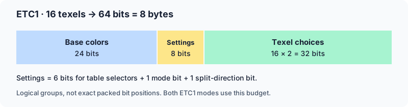
- 24 bits: describe the two base colors.
- 8 bits: select the modifier tables, color mode, and split direction.
- 32 bits: each texel selects one of its half’s four offsets using 2 bits.
Why this design? Small patches of natural imagery often have similar colors with mostly brightness variation. Sharing a base color and four offsets is cheaper than storing eight separate RGB texels. Two halves accommodate a simple color boundary, while different modifier tables handle different contrast levels. Fixed-size blocks and simple arithmetic also make random texture sampling inexpensive for GPU hardware.
ETC1 Example#
In individual mode, expand each stored 4-bit channel by multiplying by 17. Then add the selected offset to every channel, clamping to 0–255. For example, A’s index 01 gives $(102,136,170)+17=\mathbf{(119,153,187)}$.
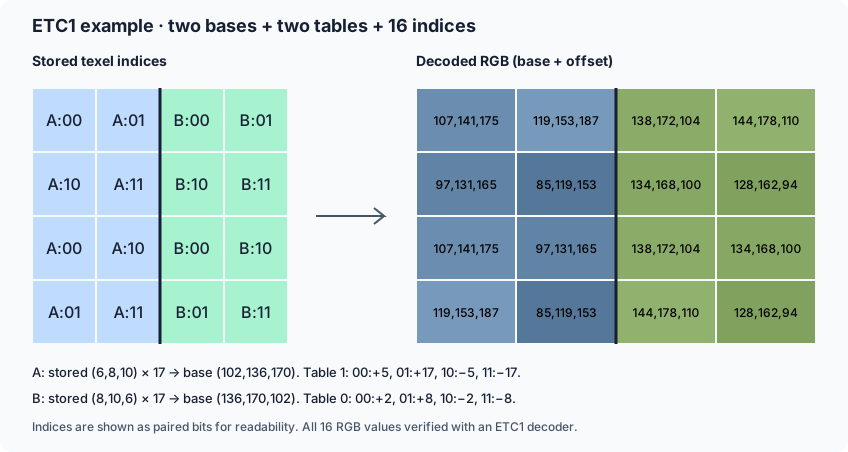
The diagram includes both stored bases, selected tables, and all 16 results. Four colors per half means at most eight colors per block.
Intended use: compact, opaque RGB color textures, especially on older mobile GPUs. Textured surfaces with local brightness variation suit this model better than independent data channels or clean multicolor gradients. The latter expose its restricted palettes and block seams. ETC1 has no planar mode; that is one of ETC2’s additions.
ETC2 Modes#
ETC2 RGB8 keeps ETC1’s two modes and adds three alternatives, chosen per 4×4 block at the same 8-byte size:
| Mode | Representation |
|---|---|
| Individual | ETC1’s two independent RGB444 bases and brightness palettes |
| Differential | ETC1’s more precise, related RGB555 bases and brightness palettes |
| T | Four colors: $C_0$, $C_1-d$, $C_1$, $C_1+d$ |
| H | Four colors: $C_0-d$, $C_0+d$, $C_1-d$, $C_1+d$ |
| Planar | Three RGB676 anchors defining a spatial color ramp |
Why add modes? ETC1’s fixed halves struggle with mixed hues and smooth ramps:
- T/H: handle color groups such as red petals against green leaves. Any texel can select any of the four palette colors, regardless of the subblock split. Adding/subtracting $d$ changes all RGB channels equally, with clamping. T gives one group one color and the other three; H gives each two.
- Planar: replaces palette selection with horizontal and vertical color changes—better suited to skies and soft gradients.
ETC2 Block Layout#
Individual/differential keep ETC1’s layout. T/H retain texel indices; planar spends those bits on anchors instead:
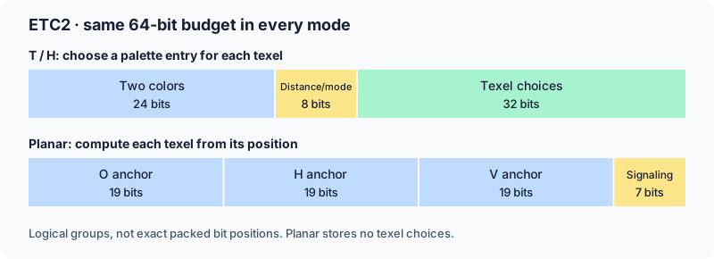
These are logical bit budgets, not exact bit positions. There is no extra mode header: diff = 0 selects individual; otherwise, test the hypothetical second ETC1 differential base before clamping. Overflow outside 0–31 in red → T, otherwise green → H, otherwise blue → planar; no overflow means differential.
Storage Size#
ETC1 and ETC2 RGB8 use 4 bits per texel. Our 192×192 example occupies 2,304 × 8 = 18,432 bytes (18 KiB), versus 108 KiB for RGB8—a 6:1 reduction, excluding headers and mipmaps. Round dimensions up to multiples of four when counting blocks.
Full ETC2 RGBA8/EAC doubles storage with a separate alpha block: 16 bytes per block, 8 bits per texel. The 1-bit punch-through variant stays at 8 bytes but has different mode rules.
Planar Mode#
Planar mode stores O at (0,0), H at (4,0), and V at (0,4). O sets the starting color; H−O and V−O define horizontal and vertical change.
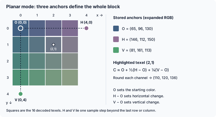
Texel coordinates run from 0 to 3, so H and V sit one step beyond the last texels. Ignoring rounding and clamping:
$$ C(x,y) \approx O + \frac{x}{4}(H-O) + \frac{y}{4}(V-O). $$Apply this independently to RGB. For example, texel (2,1) uses half the horizontal change and one quarter of the vertical change, as shown above.
Unlike BC1’s four-color line, this can produce 16 distinct colors with independent channel slopes. RGB676 anchors also have one more bit per channel than BC1’s endpoints. Smooth curved gradients often approximate a plane over a small block.
It remains lossy: anchors are quantized, outputs rounded and clamped, and neighboring blocks may not join perfectly. Curvature and encoder search quality also affect the result.
BC5#
BC5 stores two independent BC4 blocks: one for R and one for G. Each channel gets 8-bit endpoints and a 3-bit index per texel, selecting from up to eight values. The block occupies 128 bits, or 8 bits per texel.
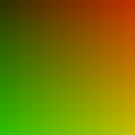
The important difference is independence: red and green no longer have to use the same interpolation index. Here red varies horizontally and green vertically; blue is zero only to visualize the two-channel data.

RMSE 0.00
RMSE 2.77

RMSE 0.82
Full 192×192 images. RMSE is measured in 8-bit R/G code values; lower is better. Scroll horizontally on narrow screens to compare all columns.
Use BC5 for two-channel data, not arbitrary RGB color. It is particularly useful for normal-map X/Y components. For unit normals on the positive-Z hemisphere, reconstruct:
$$ z = \sqrt{\max(0,1-x^2-y^2)}. $$That works because the third component is constrained, not because BC5 somehow preserves blue. Compression errors may still require renormalization. For just one scalar gradient, BC4 provides the same independent-channel model at 4 bits per texel.
BC7#
BC7 stores RGB/RGBA in 128-bit 4×4 blocks: 8 bits per texel. Its eight modes trade bits between endpoint precision, interpolation choices, and separate color groups.
Interpolation#
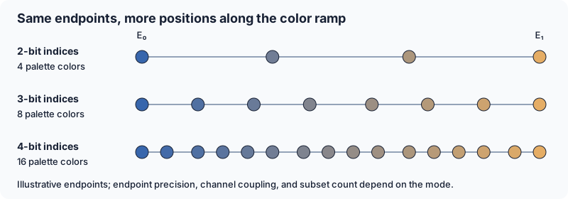
Each texel selects a weight between two endpoints, $E_0$ and $E_1$. For expanded 8-bit endpoint components:
$$ C=\left\lfloor\frac{(64-w)E_0+wE_1+32}{64}\right\rfloor. $$A 2-, 3-, or 4-bit index selects from 4, 8, or 16 fixed weights, respectively. For example, the 2-bit weights are $\{0,21,43,64\}$: approximately the endpoints and the one-third/two-thirds positions. More choices can reduce steps along a gradient; more endpoint precision helps place the ramp accurately in the first place.
Subsets#
A subset is a group of texels sharing an endpoint pair. Multi-subset modes choose a predefined partition pattern—not necessarily a rectangular split. Each subset gets its own color ramp.
Subset Examples#
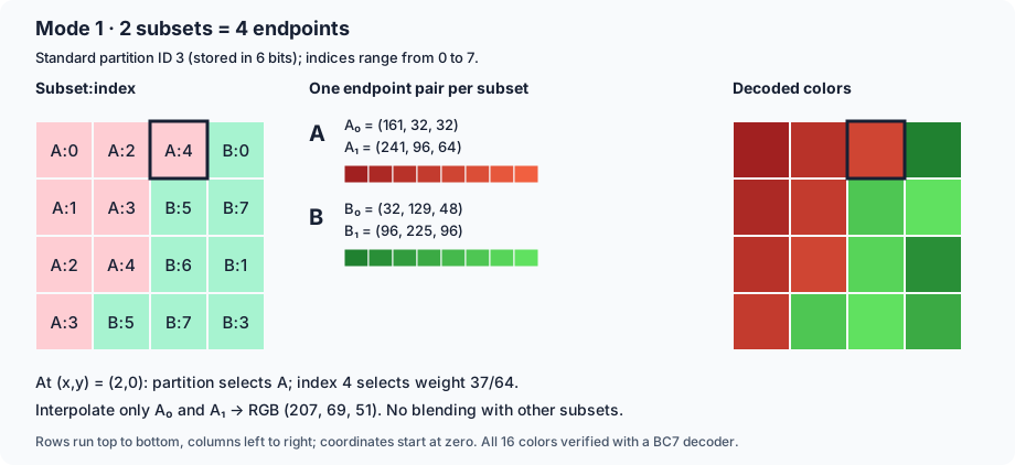
BC7 stores two endpoints per subset, not always two per block. These examples use actual standard partition patterns. Each left-hand cell shows subset:interpolation index; the right-hand grid shows the decoded result.
Two subsets, mode 1: partition ID 3 assigns the red group A and green group B along a stepped boundary. It needs four endpoints: A₀/A₁ and B₀/B₁. At (2,0), the partition selects A; index 4 selects weight 37/64 between A’s endpoints, giving RGB (207,69,51).
Three subsets, mode 2: partition ID 0 adds blue group C, requiring six endpoints. At (1,2), the partition selects C; index 2 selects weight 43/64 between C’s endpoints, giving RGB (77,133,220).
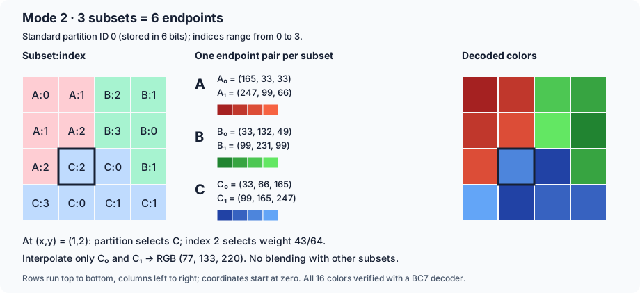
The encoder chooses a pattern from the mode’s allowed table—it cannot assign subsets arbitrarily per texel. Once the subset is known, the texel’s index selects a color only from that subset’s ramp, never by blending all four or six endpoints. Both examples are complete 16-byte blocks, verified against a BC7 decoder.
Mode Summary#
| Mode | Subsets / channels | Palette choices per texel | Intuition |
|---|---|---|---|
| 0 | 3, RGB | 8 | Fit three color groups with several shades each; coarser endpoints and only 16 partition patterns |
| 1 | 2, RGB | 8 | Balance endpoint precision and shading detail for two color groups |
| 2 | 3, RGB | 4 | Fit three groups with fewer shades; offers 64 partition patterns versus mode 0’s 16 |
| 3 | 2, RGB | 4 | Spend more on endpoint precision, less on shades; useful for two nearly flat color groups |
| 4 | 1, RGB + separate scalar | 8 / 4, assignable | Let one channel vary independently, giving either stream the finer palette |
| 5 | 1, RGB + separate scalar | 4 / 4 | More precise endpoints than mode 4, but fewer interpolation choices |
| 6 | 1, RGBA together | 16 | Prioritize a finely sampled ramp; a good candidate for smooth, correlated channel variation |
| 7 | 2, RGBA together | 4 | Fit two color/alpha groups when one RGBA ramp is insufficient |
Modes 0–3 imply opaque alpha. In modes 4/5, the separate scalar is normally alpha, but a channel swap can make it R, G, or B instead. For example, opacity can change without forcing RGB to move along its ramp. In 6/7, all four channels share one index per texel, so they move together within each subset.
Some modes also use a P-bit: an extra low bit shared across an endpoint’s channels, sometimes also across its endpoint pair. It improves endpoint precision cheaply, but does not give every channel a freely chosen extra bit.
BC7 Block Layout#
Every mode spends the same 128 bits, but divides them differently. Two examples:
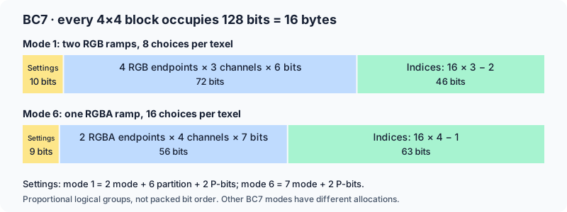
Mode 1 spends more on endpoints for two RGB ramps; mode 6 spends more on indices for one finely sampled RGBA ramp. Settings include the mode prefix, any partition selector, and P-bits. The index totals are slightly smaller than 16 × index width: one designated texel per subset omits its highest index bit, with endpoint ordering making that bit redundant.
For smooth gradients: mode 6 offers more intermediate values; partitions help when one color line is insufficient; modes 4/5 can decouple one channel. These are alternative fits, not quality levels—the encoder chooses per block.
BC7 has no ETC2-style spatial planar mode: even its 16-color palette is still an endpoint ramp. Its added flexibility reduces RGB RMSE to 0.27 here, versus BC1’s 2.31, but remains lossy and costs twice as many bits.
ASTC#
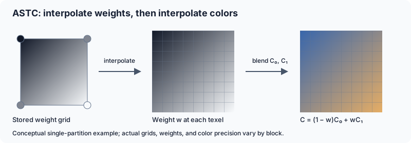
ASTC stores 128 bits per block, but lets us choose the block footprint: a larger footprint spreads those bits across more texels. The footprint is fixed for the texture, not chosen independently per block. Within each block, the encoder adapts how those bits are spent.
Like BC7, it blends endpoints. For one partition, conceptually:
$$ C(x,y) = (1-w(x,y))C_0 + w(x,y)C_1. $$The main difference is how it represents $w(x,y)$: ASTC can store a lower-resolution weight grid, then interpolate weights at texel positions. A smooth ramp may need only a few stored weights, leaving more bits for accurate endpoint colors.
Adaptive Encoding#
| Choice | Intuition |
|---|---|
| Endpoint encoding | Use a suitable representation—such as luminance, RGB, RGBA, or base-plus-offset—to avoid spending bits on unnecessary color information |
| 1–4 partitions | Give different color groups their own endpoint pairs, rather than forcing everything onto one ramp |
| Weight-grid density and precision | Use fewer weights for smooth changes, more for detail; trade weight accuracy against endpoint accuracy |
| Dual-plane weights | Let one channel, such as alpha, vary independently of the others; unavailable with four partitions |
For example, with endpoints $(40,80,120)$ and $(200,160,80)$, a weight of $1/4$ gives $(80,100,110)$ before codec-specific rounding. The grid determines that weight; the texel does not need a separately stored palette index.
ASTC Block Layout#
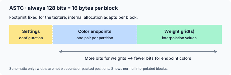
- Settings: weight-grid configuration, partition count/pattern, endpoint encoding, and any dual-plane channel selection.
- Endpoints: quantized color values for each partition’s ramp.
- Weights: one or two quantized grids, expanded to texel weights during decoding.
Unlike BC7’s small set of fixed mode layouts, ASTC varies the endpoint/weight allocation. More partitions or weights leave fewer bits for other data. Its compact integer encoding supports non-power-of-two precision levels too—for example, three values with five possible levels fit in 7 bits, rather than three separate 3-bit fields totaling 9.
An ASTC weight plane is not ETC2’s planar mode. A single weight field still ties the color channels together along an endpoint line; smooth weight interpolation alone does not represent every RGB plane exactly.
RMSE 0.00

RMSE 0.27

RMSE 0.18

RMSE 0.44

RMSE 0.61
Full 192×192 images. RMSE is measured in 8-bit RGB code values; lower is better. Scroll horizontally on narrow screens to compare all columns.
| ASTC footprint | Bits per texel | RGB RMSE in this test |
|---|---|---|
| 4×4 | 8.00 | 0.18 |
| 6×6 | 3.56 | 0.44 |
| 8×8 | 2.00 | 0.62 |
This simple gradient compresses particularly well, even at larger footprints. Do not generalize that result to detailed or curved content. Larger blocks cover more variation with the same 128 bits and generally make faithful reconstruction harder. Test several footprints on the actual asset.
Conclusion#
For smooth gradients, choose a format that preserves small changes rather than just one that compresses well on detailed textures. These are useful starting points, subject to support on the target GPU:
| Content / target | Suggested format | Why |
|---|---|---|
| RGB/RGBA on desktop and console with BC7 support | BC7, 8 bits per texel | Finer interpolation and more flexible endpoint fitting than BC1; a strong default when gradient quality matters |
| RGB/RGBA on ASTC-capable devices | ASTC 4×4 for quality; test 6×6 or 8×8 to reduce storage | Flexible endpoint and weight representations; larger footprints worked well here, but need validation on the actual gradient |
| Opaque RGB on ETC2-capable devices at 4 bits per texel | ETC2 RGB8, with an encoder that considers planar mode | Planar mode directly fits spatial color ramps, making it particularly suitable for locally planar gradients |
| Two independent scalar channels | BC5, 8 bits per texel | Each channel gets its own endpoints and interpolation indices; not a replacement for RGB compression |
| One scalar channel | BC4, 4 bits per texel | Avoids spending bits on unused color channels and fits the scalar independently |
BC1 and ETC1 are compatibility or budget choices, not first choices for clean gradients. Their restricted palettes can expose banding and block seams. ETC2 planar mode improves this at the same RGB bitrate, while BC7 and ASTC offer other quality/storage tradeoffs. None guarantees artifact-free results.
Check the decoded texture at its intended display size, with the actual color space, filtering, and mipmaps. Use the magnified error views to diagnose differences, not as the sole quality criterion. The measurements above favor this particular test image and encoder configuration; they are not a universal format ranking.
If visible artifacts remain unacceptable, keep the gradient uncompressed at suitable precision, or generate it procedurally when practical. Compression is only worthwhile if its savings justify the visible error.